Author: Danjue Chen, Jorge A.Laval, Soyoung Ahn, Zuduo Zheng
Abstract
The paper investigated the impact of driver behavior on traffic hysteresis in traffic oscillations. The driver's behavior impacts the occurrence and the type of traffic hysteresis. The reaction time driver to deceleration wave is highly correlated with traffic hysteresis. The research suggests using the different car-following models by the different stages of an oscillation.
The findings of this research can be explained below.
- The paper shows the generation mechanisms of traffic hysteresis in traffic oscillations.
- The paper showed that traffic hysteresis is correlated with driver behavior in oscillation.
- The paper showed that driver behavior varies with the development stage of traffic oscillations.
- The paper showed that the behavior change of driver results in a different distribution of hysteresis loops.
Introduction
In general, traffic hysteresis is retardation in speed recovery. Newell (1965) argued that hysteresis results from the asymmetry between acceleration and deceleration. Zhang (1999) used three phases to describe traffic flow: acceleration, deceleration, and strong equilibrium. Yeo and Skadarbonis (2009) defined five traffic states: free-flow, acceleration, deceleration, coasting, and stationary. Same as Newell, they also suggest the asymmetry between acceleration and deceleration causes traffic hysteresis.
The paper focuses on hysteresis in stop-and-go traffic only. However, hysteresis happens in other types of traffic flow too. Yeo and Skabardonis (2009) observed hysteresis even in stable speed traffic flow.
The paper uses the "Next Generation Simulation project" (NGSIM, 2006) data. While the data is collected in the 6-lane 2100-foot segment, they used the data of lane one from 7:50 to 8:05 am, on June 15, 2005. The figure below illustrates the oscillations they studied. The red line shows how the speed of the vehicle drops by oscillations.

Background
$$\tau={1\over wk} \ and \ d={1\over k}$$
The variable $\tau$ is the wave trip time between two consecutive drivers (time shift), and $k$ is the jam spacing. Then $d$ becomes a space shift. $w$ indicates the wave speed, and $k$ is jam density. The individual driver can be denoted as subscript $i$. Detailed information is described below.

Laval and Leclercq (2010) found out that wave trip time and space shift varies, and it was measured by ${\tau_i(t)}/ {\tau}$.
$$\eta_i(t) = \tau_i(t)/\tau$$
$\eta_i(t)$ deviated from the constant value when the non-equilibrium flow started. The beginning and ending points of the response to an oscillation are denoted by $t^0$ and $t^1$, respectively. It is noteworthy that the response refers to the change of $\eta_i(t)$ rather than the physical action such as acceleration or deceleration. By the value of $\eta^0_i$, the type of driver was categorized: originally aggressive (OA) if $\eta^0_i << 1$, originally timid (OT) if $\eta^0_i >> 1$, and originally Newell (ON) if $\eta^0_i ~ 1$.

The hysteresis was analyzed in $v-\eta$ plot. In the $v-\eta$ plot, they capture five types of hysteresis: clockwise (CW) loop, counter clock-wise (CCW) loop, overlap, straight line, and multiple loops.


The figure below is the example of the concave pattern with CW loop; (b) example of a convex pattern with CW loop; (c) illustration of CW+ and CW- hysteresis loop.

Discussions
From a modeling perspective, their findings indicate that the oscillation development stage should be taken into account
when modeling the driver's car-following behavior. The statistical results (which are not included in this article) suggest that driver behavior varies with the development stage of traffic oscillations. In particular, drivers' preference of reaction pattern and response scenario varies in different development stages.
In order to take the behavior change into account in a simulation model, one possibility is to evaluate the leader's speed as a proxy for the oscillation development stage. For example, once the leader's speed reaches zero, the oscillation stage is fully-developed, while before that instance, the stage is growth. They also find it necessary to capture the response scenario when describing the driver's car-following behavior because that will affect the traffic hysteresis generated.
Fortunately, their empirical results suggest that the reaction patterns mainly occur in two response scenarios, early or late response. Therefore, one may assume that early response is initiated whenever the deceleration wave is triggered, and the late response starts at the beginning of the acceleration process. This can be included in the behavioral model without adding additional parameters.
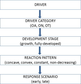
The procedure for numerical simulation is presented in the figure above. Driver behavior is determined in four layers: (i) the proportion of each driver category (OA, ON, OT), (ii) the stage of traffic oscillations (growth or fully-developed), (iii) the probability of reaction patterns (concave, convex, constant, or non-decreasing) that each driver category will adopt, which depends on the development stage of traffic oscillations, and (iv) the response scenario (early or late reaction pattern).
Reference
Chen, Danjue, Jorge A. Laval, Soyoung Ahn, and Zuduo Zheng. "Microscopic traffic hysteresis in traffic oscillations: A behavioral perspective." Transportation Research Part B: Methodological 46, no. 10 (2012): 1440-1453.
'Transportation' 카테고리의 다른 글
| Graph Attention Networks(GAT)와 교통분야에서의 응용 (0) | 2022.05.11 |
|---|---|
| 우리나라의 지능형교통체계 표준 노드링크 구축 기준 및 적용 (0) | 2022.04.24 |
| 서비스링크 기준의 인접 행렬 만들기 (0) | 2022.04.24 |
| QGIS와 python으로 지도에서 원하는 링크 선택하기 (0) | 2022.04.24 |
| 서울시 교통정보 시스템과 국가 표준 노드 링크 체계 맞추기 (1) | 2022.04.23 |


