This article summarizes RL Course by David Silver - Lecture 2: Markov Decision Processes.
Markov Property

When we assume every data about the past is in the present state, that state has a Markov property.
The state transition matrix P contains all information about transition probability between states.
Markov Process
The sequence of states with Markov property (or Markov chain) is a Markov process. Markov process contains two elements: States and Probability matrix.
Markov Reward Process
The Markov reward process is a Markov process (or Markov chain) with values. The reward function contains an expectation of reward and a discount factor.
Return is discounted by a discount factor λ. When λ is close to 0, it means the myopic evaluation. λ close to 1 means far-sighted evaluation. Why do we need a discount factor?
1. It is mathematically convenient to discount rewards.
2. It Avoids infinite returns in cyclic Markov processes.
3. We have uncertainty that the future may not be fully represented.
4. If the reward is financial, immediate rewards may earn more interest than delayed rewards.
5. Animal/human behavior shows a preference for immediate reward.
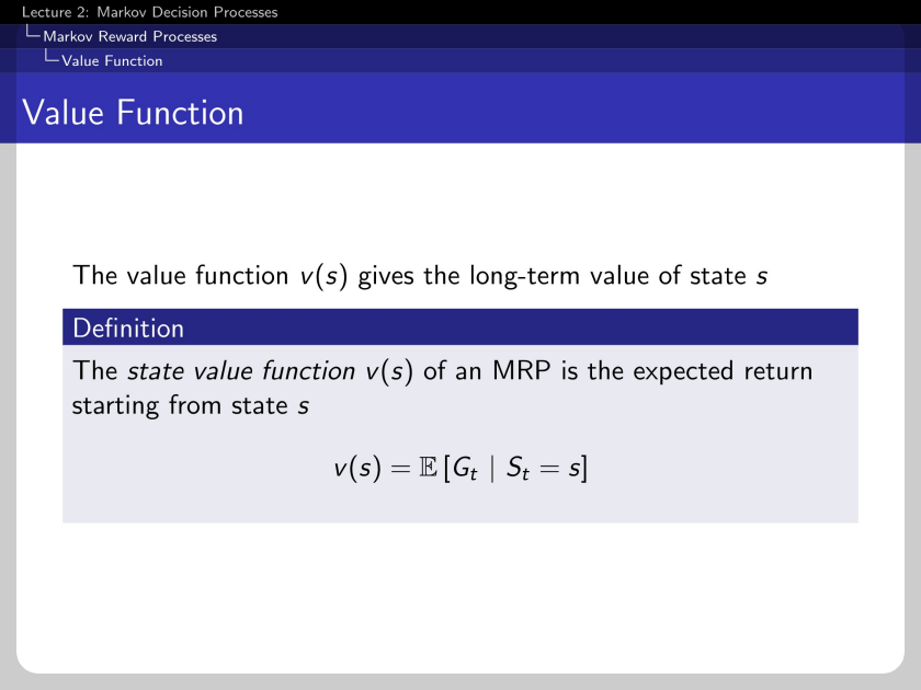
The value function v(s) gives the long-term value of state s; in other words, it is an expected return started from state s.
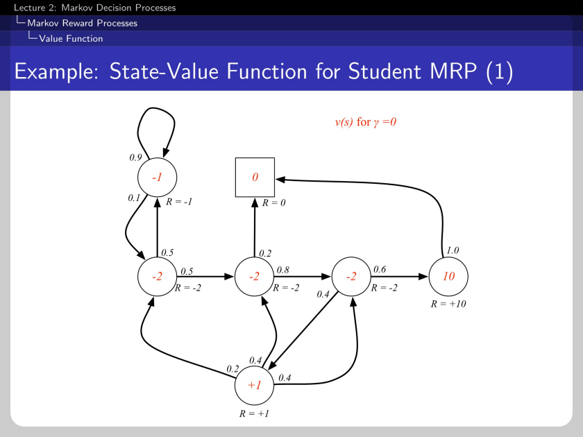
Here, we can check the left-top cornered circle with the value of -1 because it is too myopic that it only receives its reward.
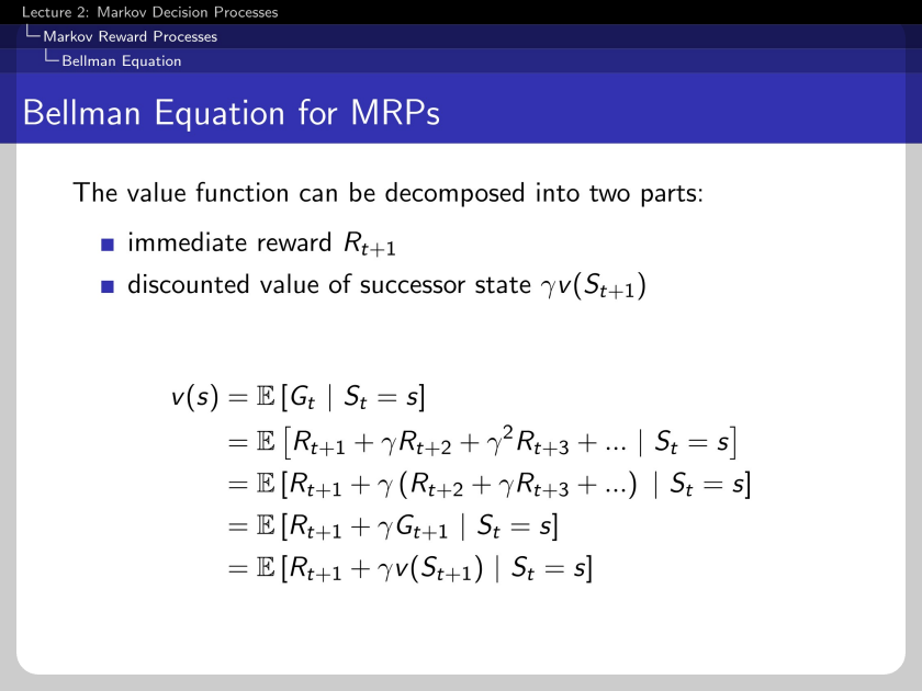
Bellman Equation for MRP has two parts: immediate reward Rt+1 and the discounted value of the successor state.
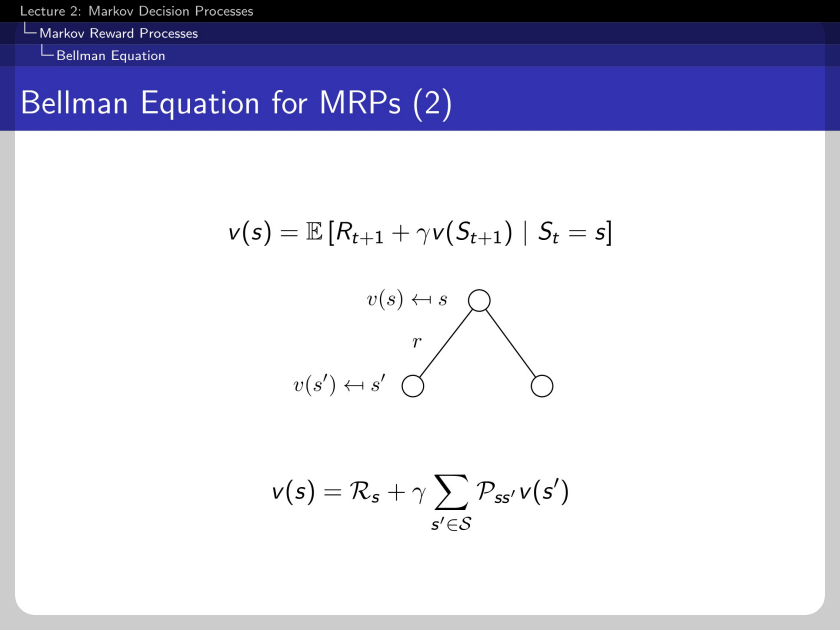
The graphical representation of the Bellman equation can be written as above.
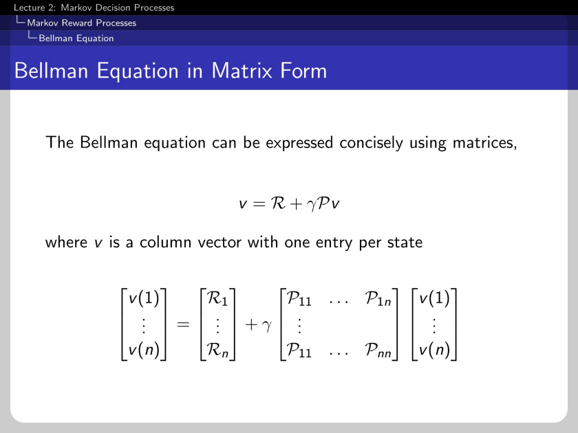
The equation can be expressed in the matrix form, where n represents a total number of possible states.
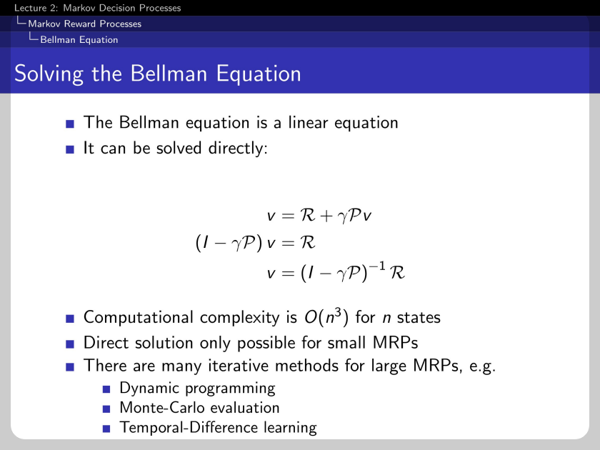
The Bellman equation is a linear equation; thus can be solved in a direct solution.
Markov Decision Process
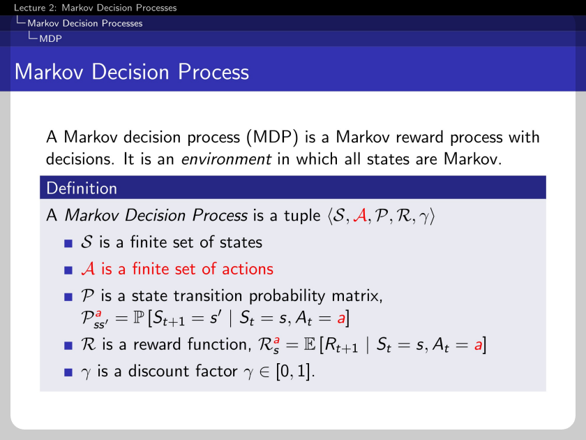
The difference between the Markov decision process and the Markov reward process is the existence of actions.
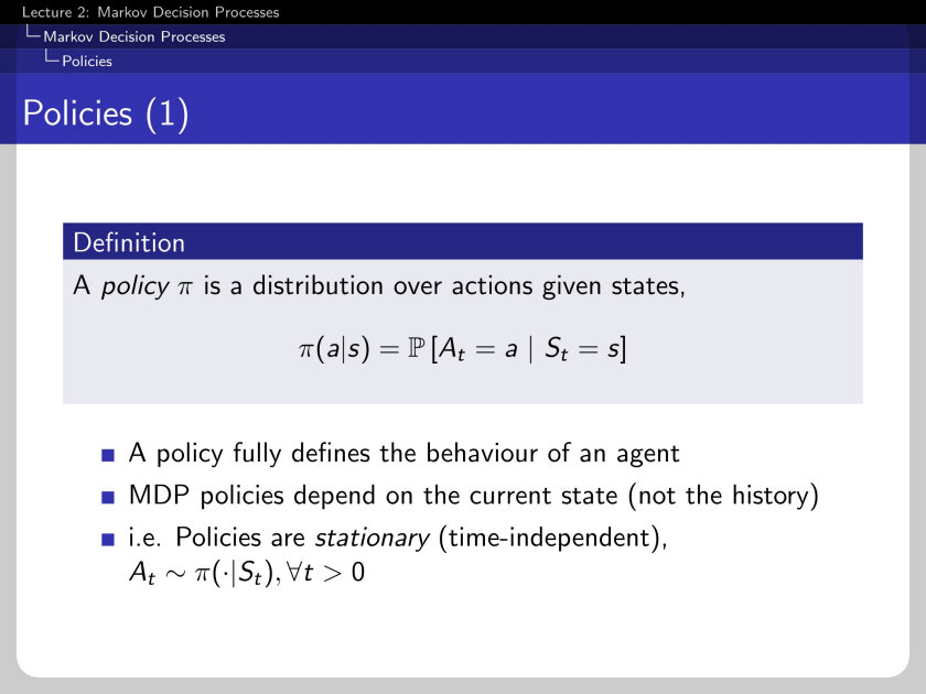
The action of MDP can be generalized into policy. The policy π is a distribution over actions given states.
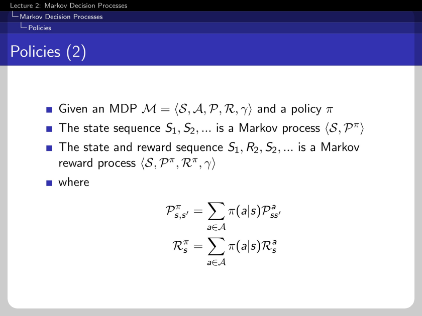
When we sum up all possible consequences from action a, the MDP is transformed into MRP.
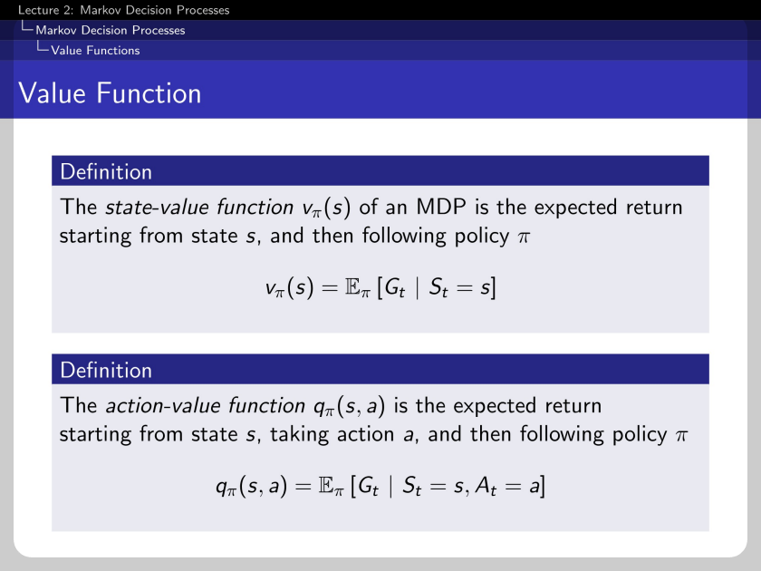
There are two value functions: The sate-value function and the action-value function. State-value function is an expected return starting from state s. The action-value function is the expected return starting from state s, taking action a, and following policy π.
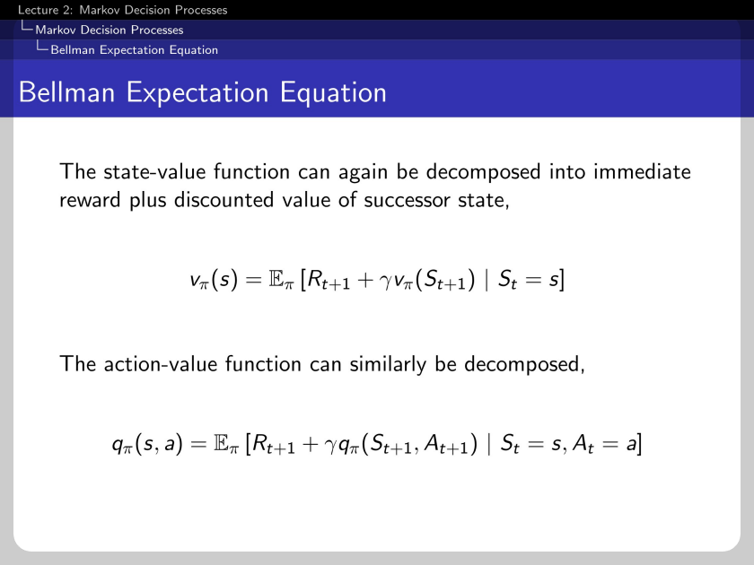
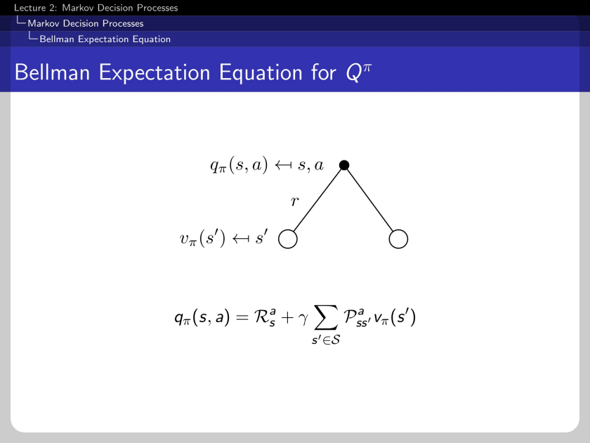
The action-value function can be decomposed into immediate reward and discounted action-value of successor action-sate pair.
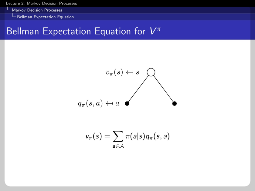
The state-value function and the action-value function have connectivity.
The connectivity between two functions can be expressed vice-versa.
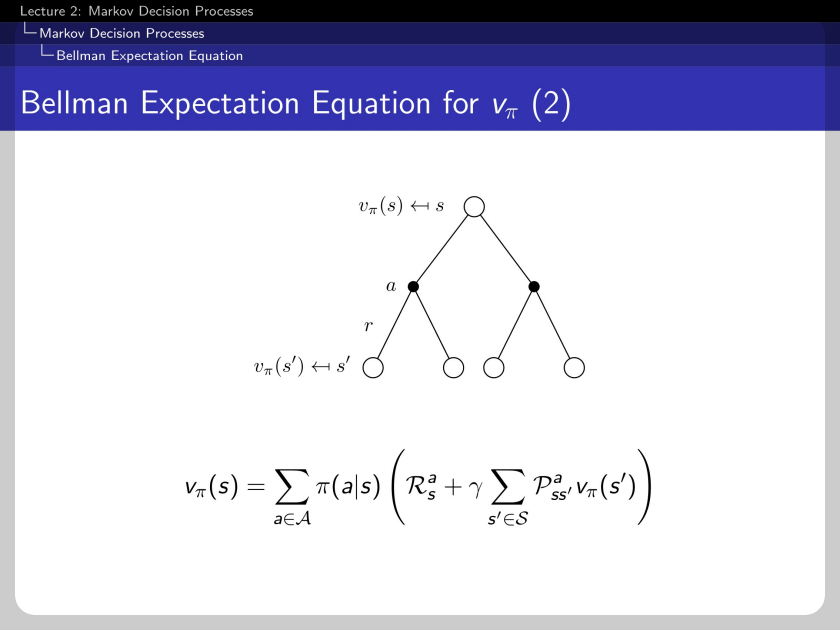
Combining two connectivity, the Bellman expectation equation for vπ can be transformed as above. The equation contains the state-value function and policy π.
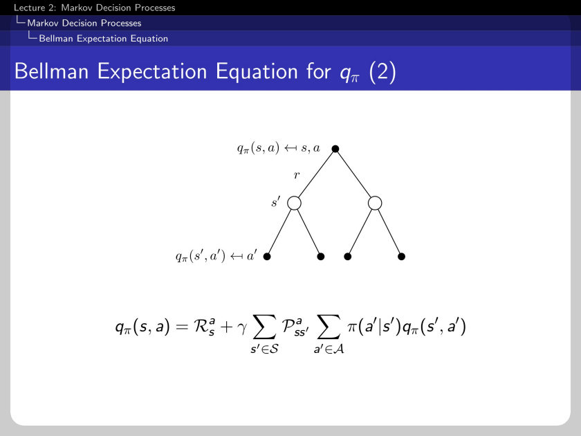
The transformation can also be applied to the Bellman expectation equation for qπ.
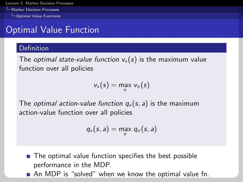
Now we define the optimal value function. The optimal state-value function is the maximum value function of overall policies. This means the maximum value function chooses argmax policy π for its value. This is the same for the optimal action-value function.
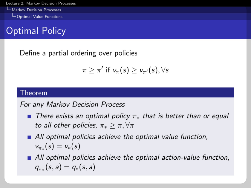
The optimal policy has to maintain the characteristics above, which is quite trivial. Furthermore, the optimal policy has to be better than or equal to every other policy in every state. And the optimal policy achieves the optimal value function. Lastly, the optimal policy achieves the optimal action-value function.
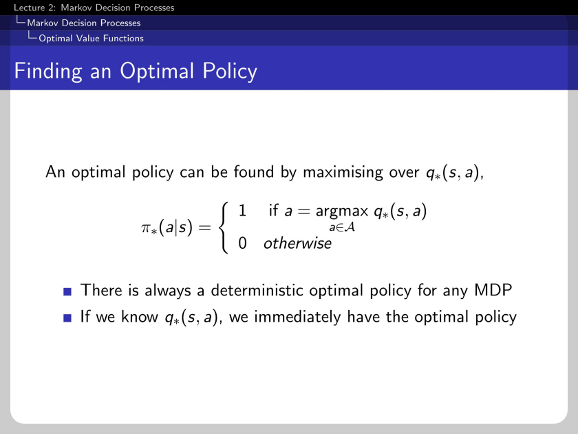
The optimal policy is a one-hot action vector. It is deterministic, and figuring out the optimal action-value function leads to the optimal policy.
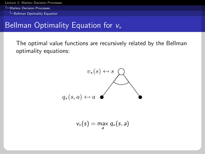
The Bellman optimality equations recursively relate to the optimal value function.
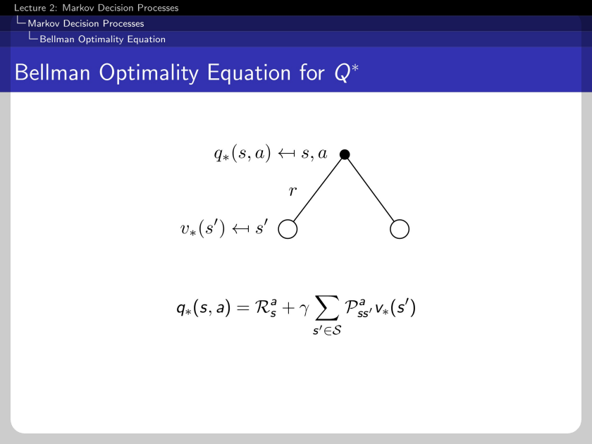
This is another direction of recursively related Bellman optimality equations.
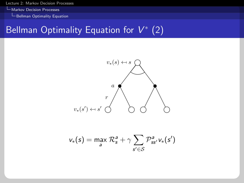
Here the only difference between the Bellman expectation equation is the existence of the max function.
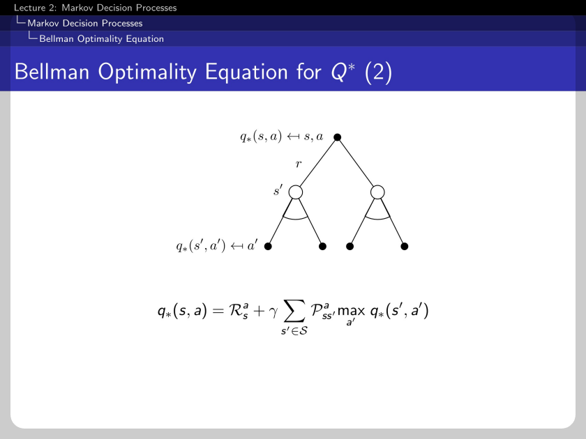
The same max function can be applied to the action-value function.
Thus the Bellman optimality equation is non-linear, and the close form does not exist in general. This is the difference between the expectation equations.
'Machine Learning > Reinforcement Learning' 카테고리의 다른 글
| RL Course by David Silver - Lecture 4: Model Free Prediction (0) | 2022.08.04 |
|---|---|
| On-Policy, Off-Policy, Online, Offline 강화학습 (0) | 2022.06.23 |
| RL Course by David Silver - Lecture 3: Planning by Dynamic Programming (0) | 2022.05.18 |
| RL Course by David Silver - Lecture 1: Introduction to Reinforcement Learning (0) | 2022.04.27 |


