This article summarizes RL Course by David Silver - Lecture 4: Model Free Prediction. This chapter will mainly discuss how to predict the value of each state. Monte Carlo and Time Difference is a two main streams algorithm.

Chapter 3 was about known MDP. Here we deal with an unknown MDP. Model-free prediction updates the value function of unknown MDP, and Model control updates the policy based on value.
Monte Carlo Reinforcement Learning

First, we will check the Monte Carlo(MC) algorithm. MC algorithm does not need MDP knowledge (transition and rewards). But it can only be applied when the environment is episodic. MC uses empirical mean return instead of expected return. It does not need to estimate because the return from MC is a true value of the return.
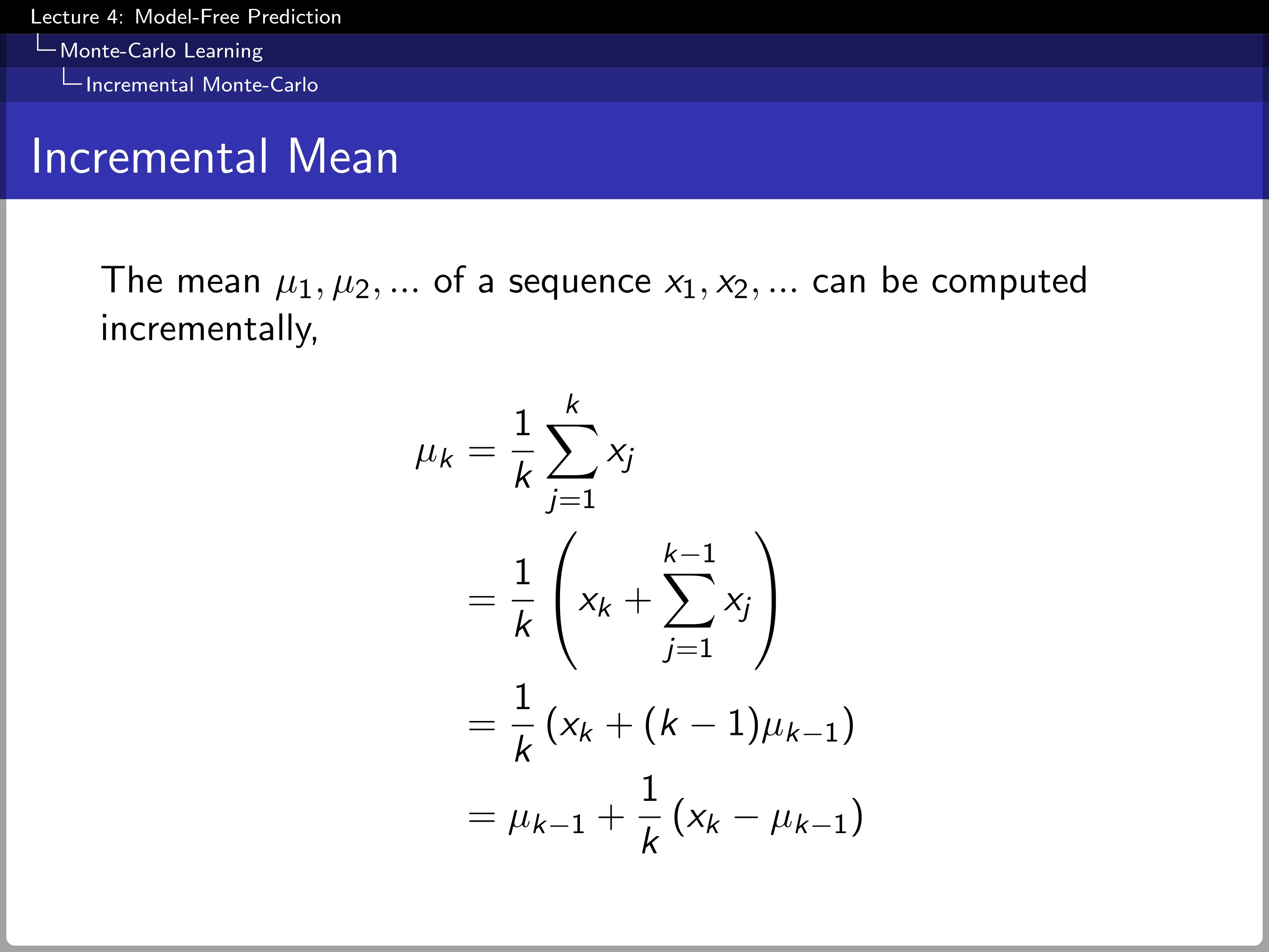
When we incrementally calculate the mean by using $1/k$ as a coefficient of $x_{k}- \mu_{k-1}$, we do not need to store the whole past value of $x_{k}$.

Changing the $k$ to the number of visit counts $N(S_{t})$, the update is transformed to $V(S_{t}) + (1/N(S_{t}))(G_{t}-V(S_{t}))$. $N(S_{t})$ can be changed into alpha for non-stationary problems.

The plane in the slide above results from the value function in Blackjack by MC.
Temporal-Difference Learning
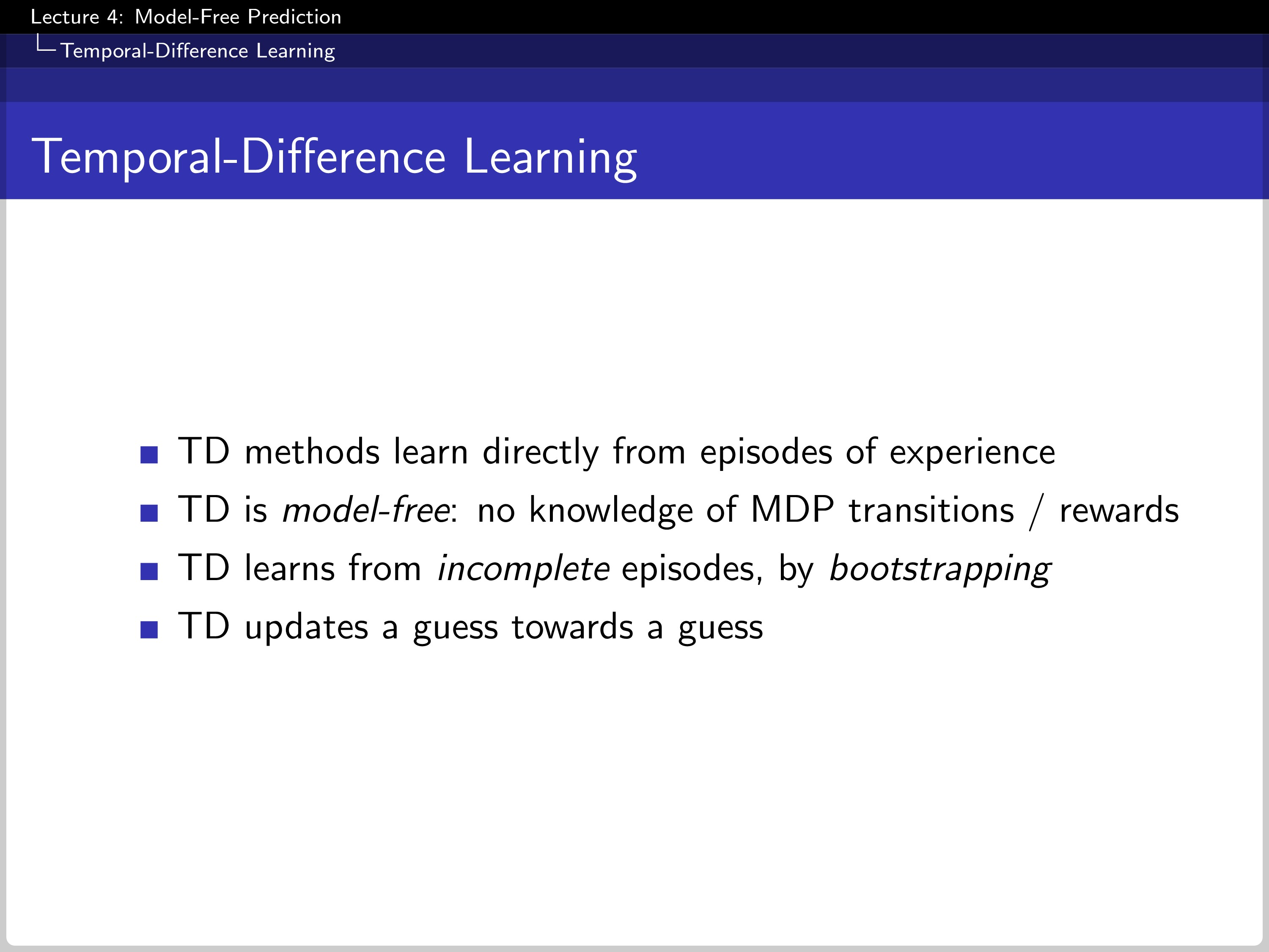
The temporal Difference(TD) algorithm learns directly from the action and reward. TD does not need knowledge of MDP like MC. TD can also learn from the incomplete episodes by bootstrapping. TD updates a guess using a guess.

The major difference between MC and TD is how they update the value of $S_{t}$. MC updates the value using actual return $G_{t}$, and TD updates the value by estimated return $R_{t+1} + \gamma V(S_{t+1})$. $R_{t+1} + \gamma V(S_{t+1})$ is also a guess, but at least it has data one step further.
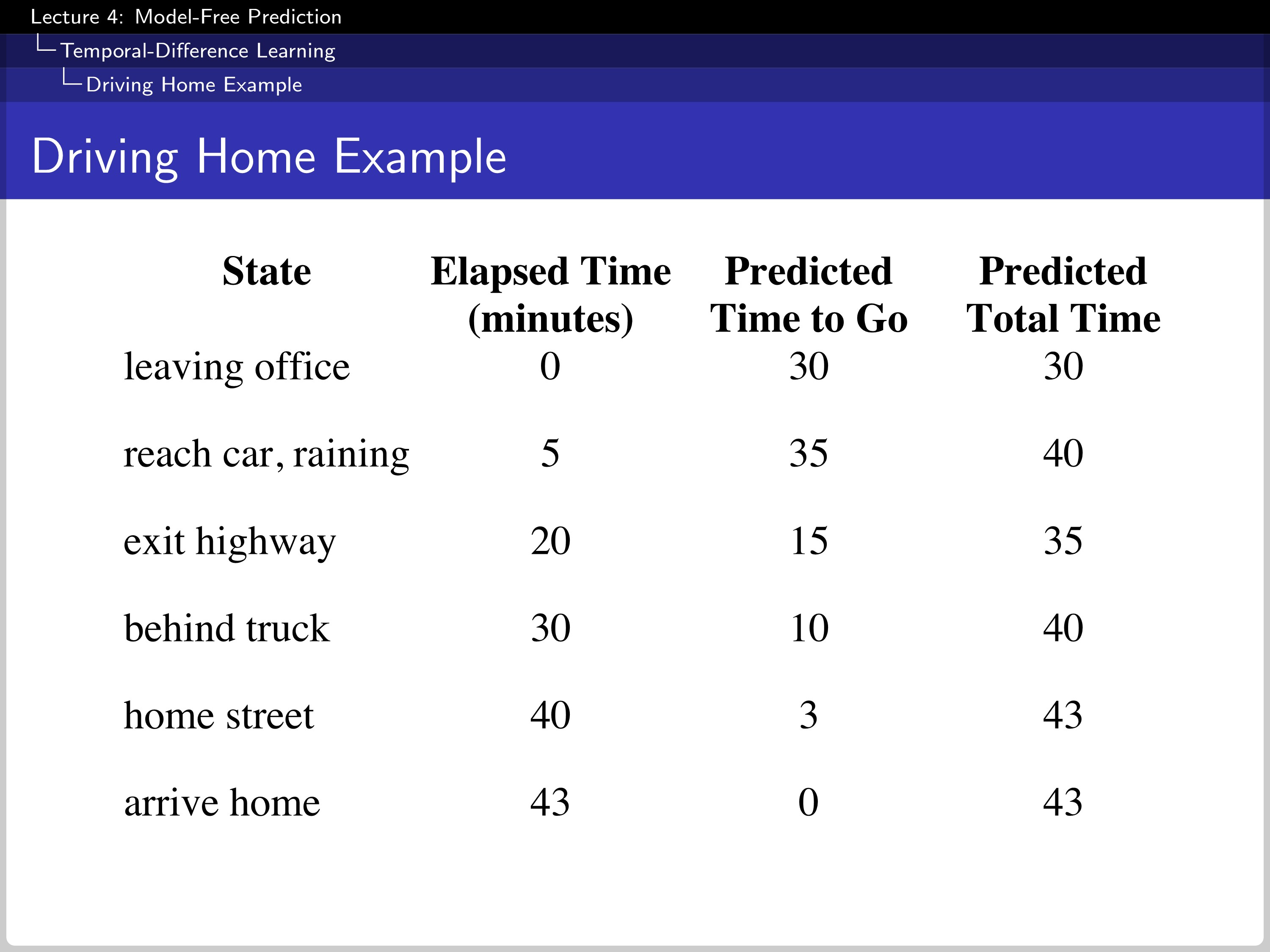
This is an example of going home from work. Every time the event happens, the expectation is updated.
Difference between MC and TD: 1. Update Process
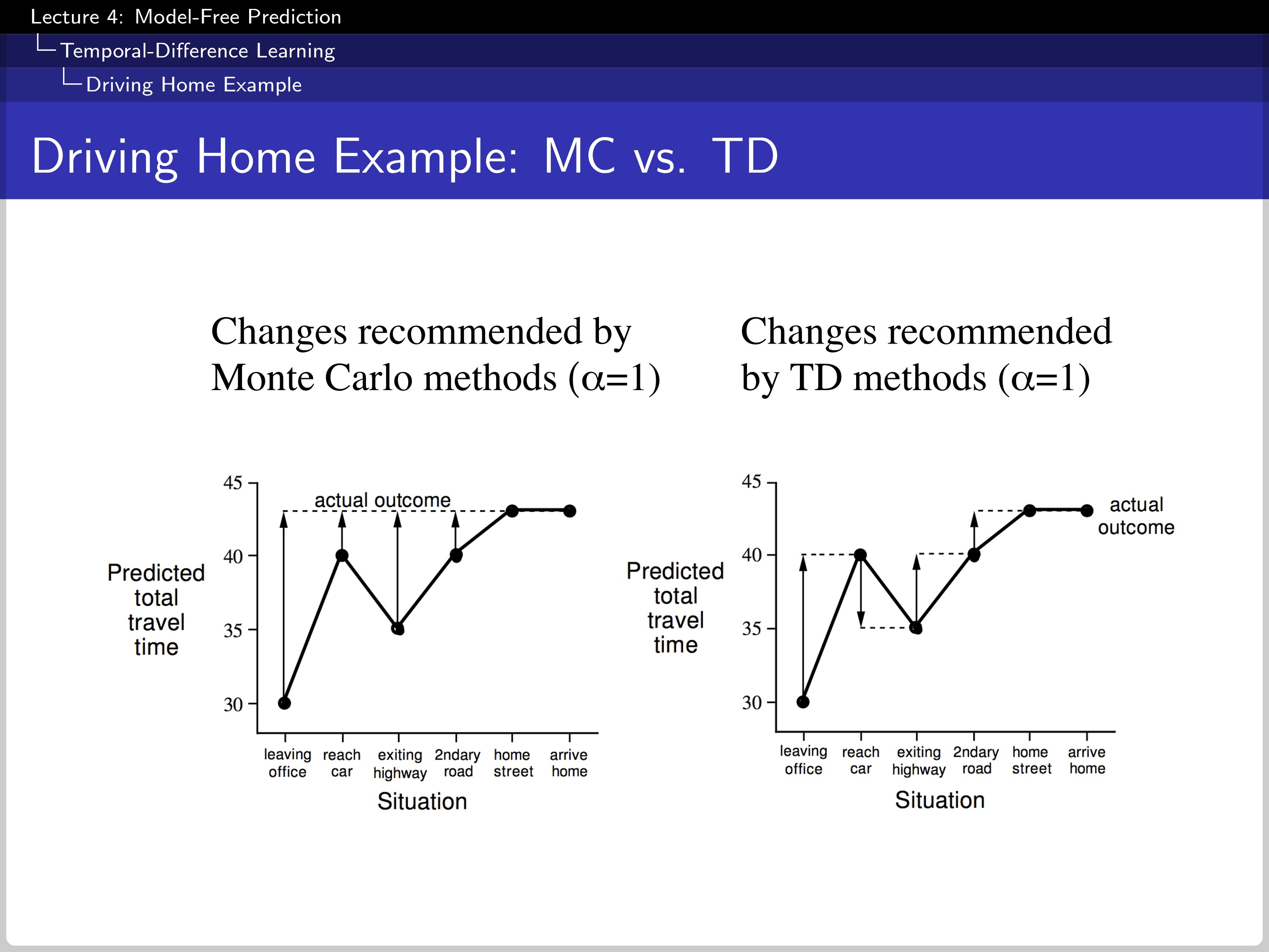
Recalling the example above, the update of MC is done by the actual outcome. However, TD updates the estimation every single time with a new prediction.
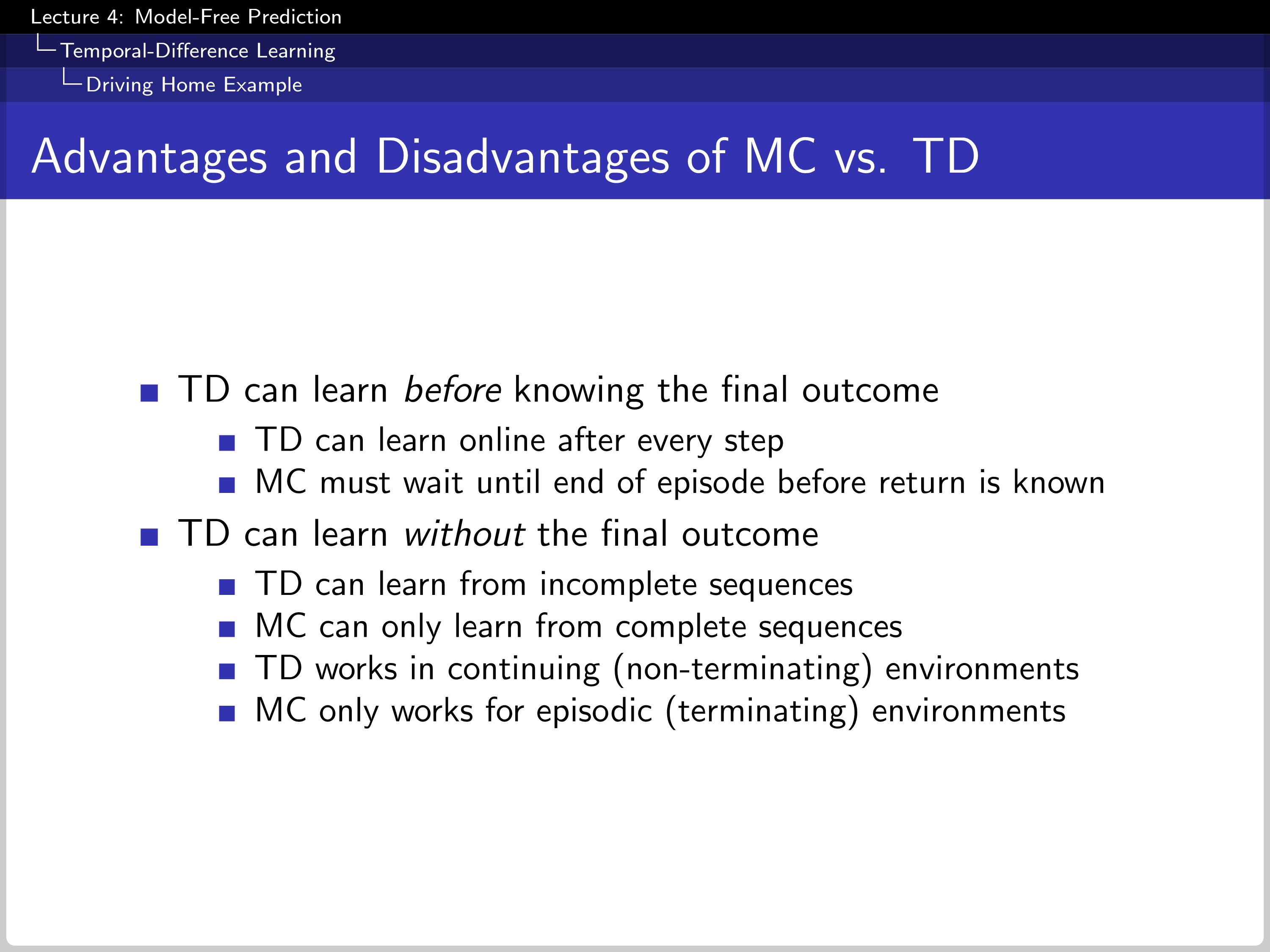
MC needs to end the whole episode to update. While TD needs only a step further. MC gives unbiased estimate of $v_{\pi}(S_{t})$.
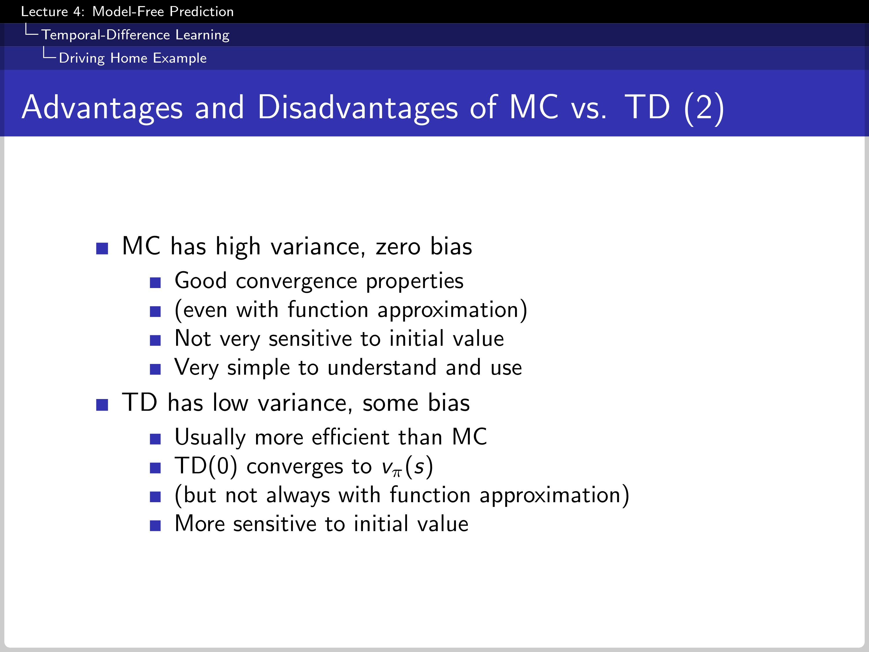
However, the TD target $R_{t+1}+\gamma V(S_{t+1})$ is a biased estimate of true $v_{\pi}(S_{t})$. So in the aspect of bias, MC has an advantage over TD. On the other hand, TD has a much lower variance.
Difference between MC and TD: 2. When There is Only a Limited Sample of MC and TD
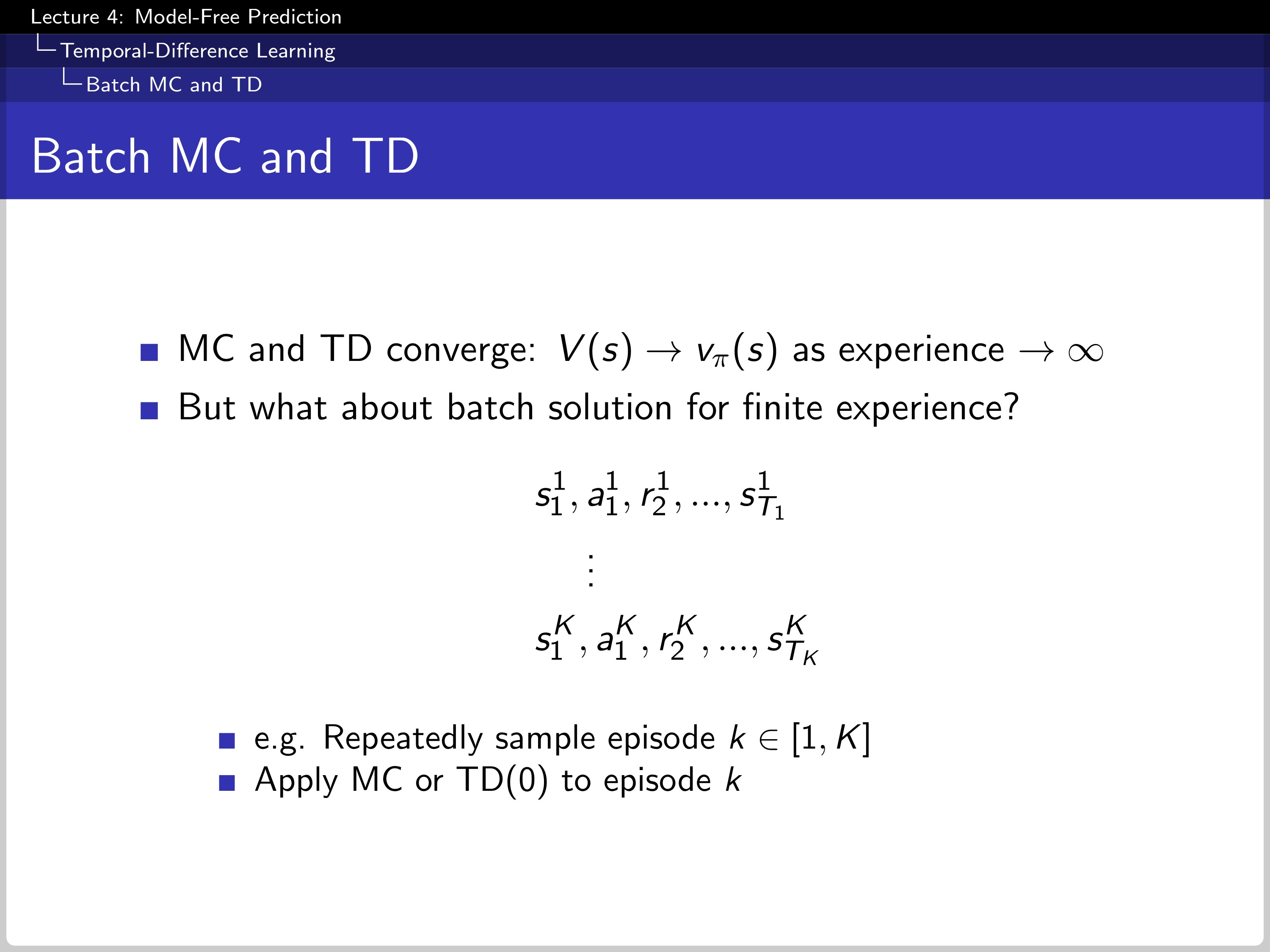
MC and TD converge when there is infinite experience. How about when the experience is limited to batch size K?
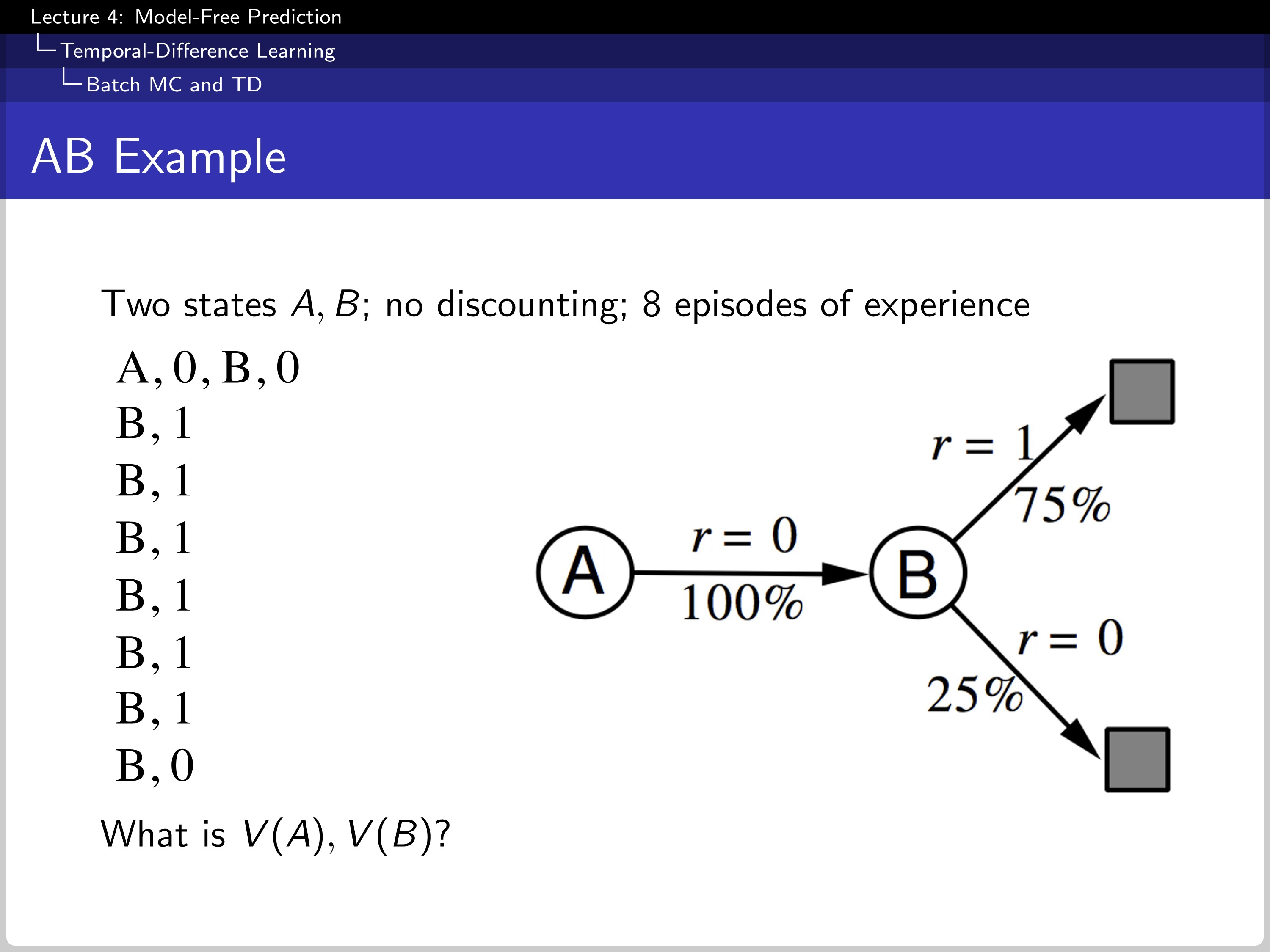
Let us figure it out with the example above. The left sequence shows the experience of the agent. The right figure is how the environment works, which means the full knowledge of the environment.
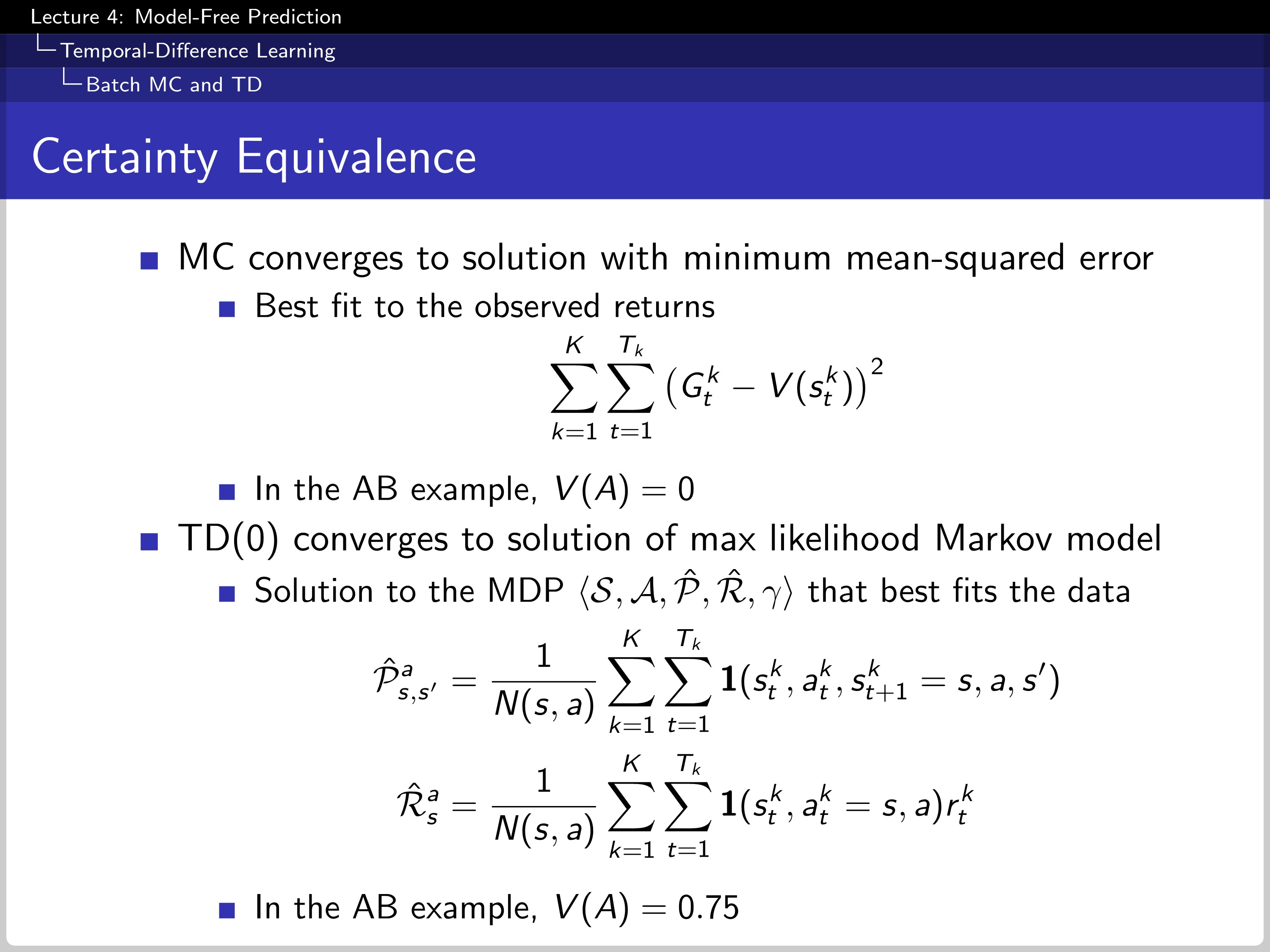
When MC and TD try to figure out the value of A, MC converges to a solution with minimum mean-squared error, and TD converges to the maximum likelihood Markov model.
- TD exploits Markov property. It is usually more efficient in Markov environments.
- MC does not exploit Markov property. Usually more effective in non-Markov environments.
Difference between MC and TD: 3. How They Backup, Bootstrap, and Sample
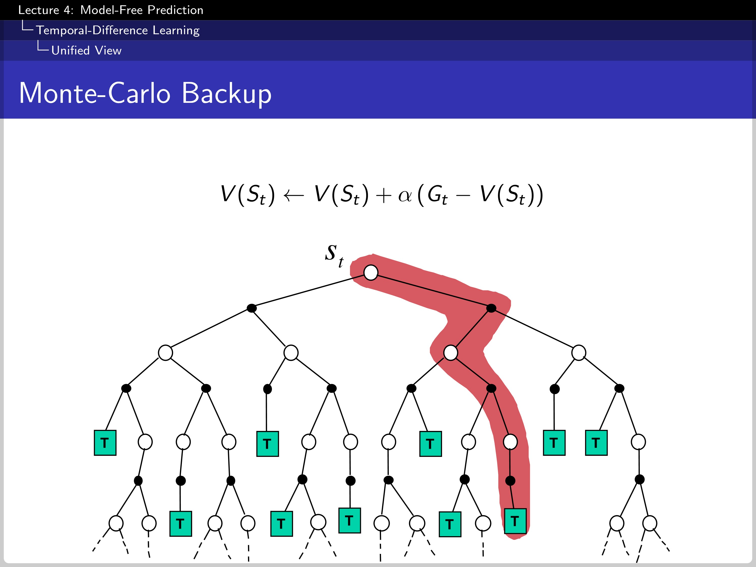
This is how MC makes a backup.
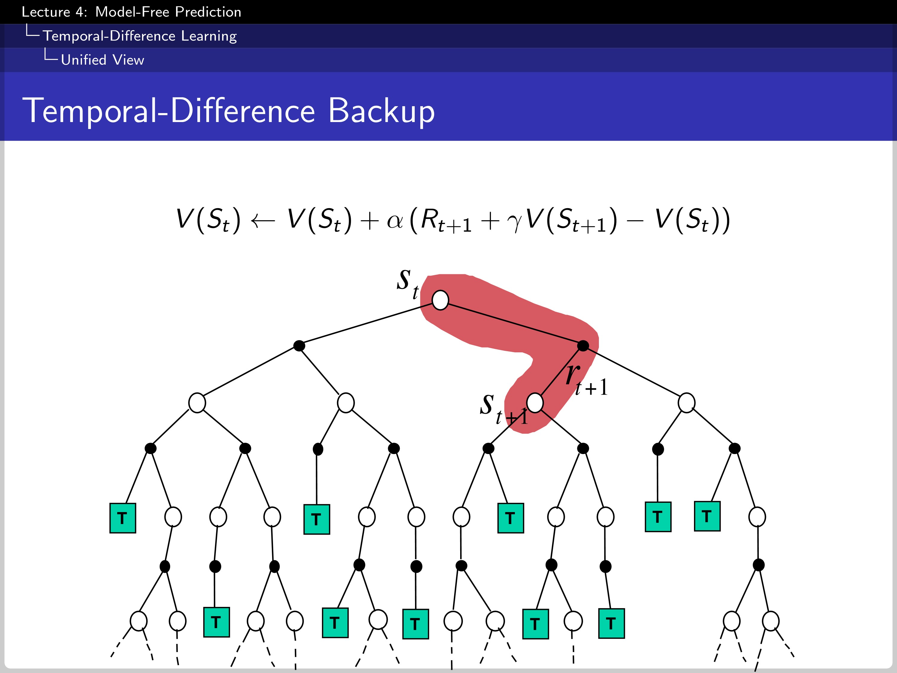
And this is how TD makes a backup. In this case, TD(0).
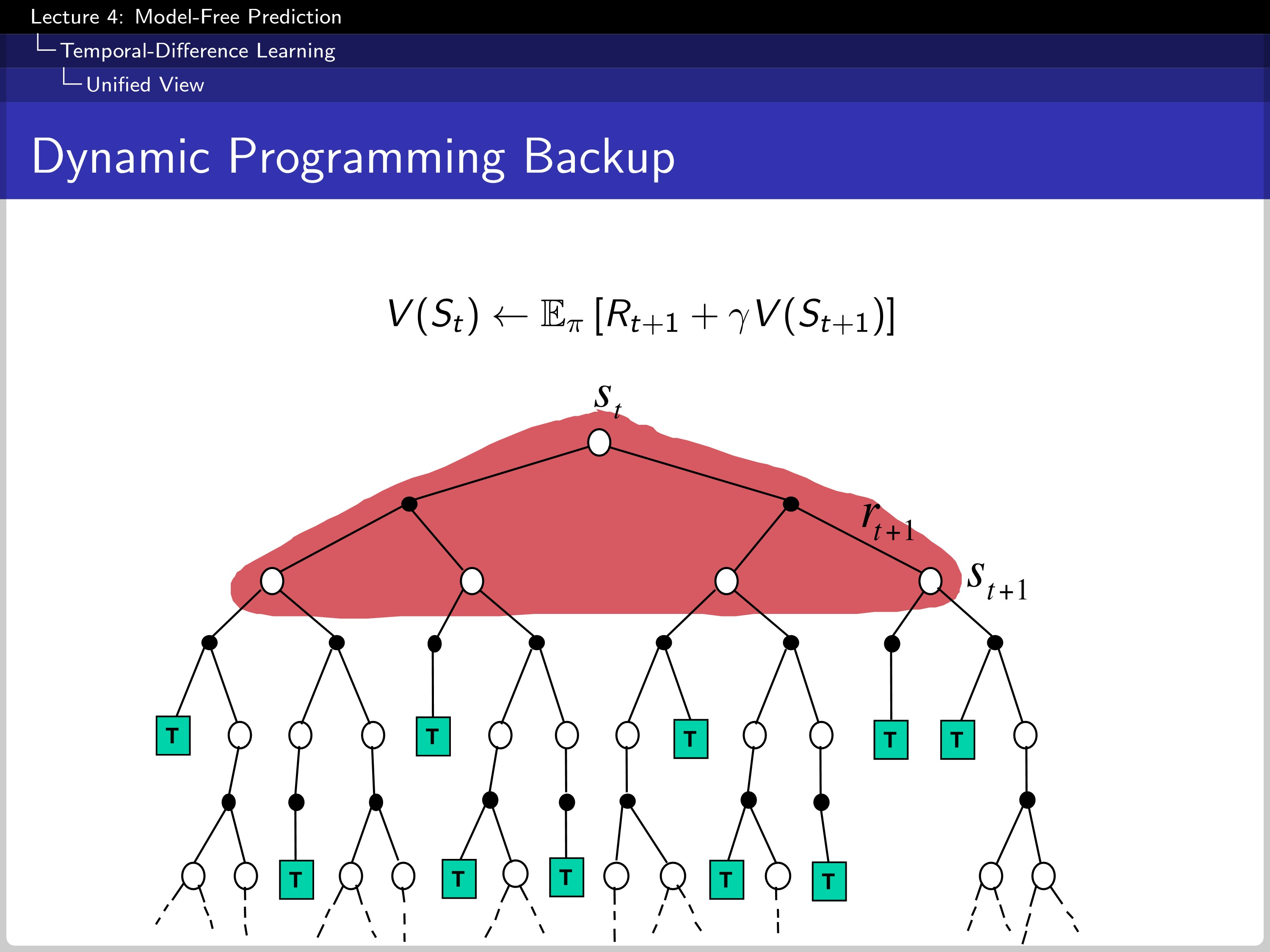
Lastly, the DP backup. Dynamic programming has full knowledge of transition probability and reward so that it can calculate the expectation.
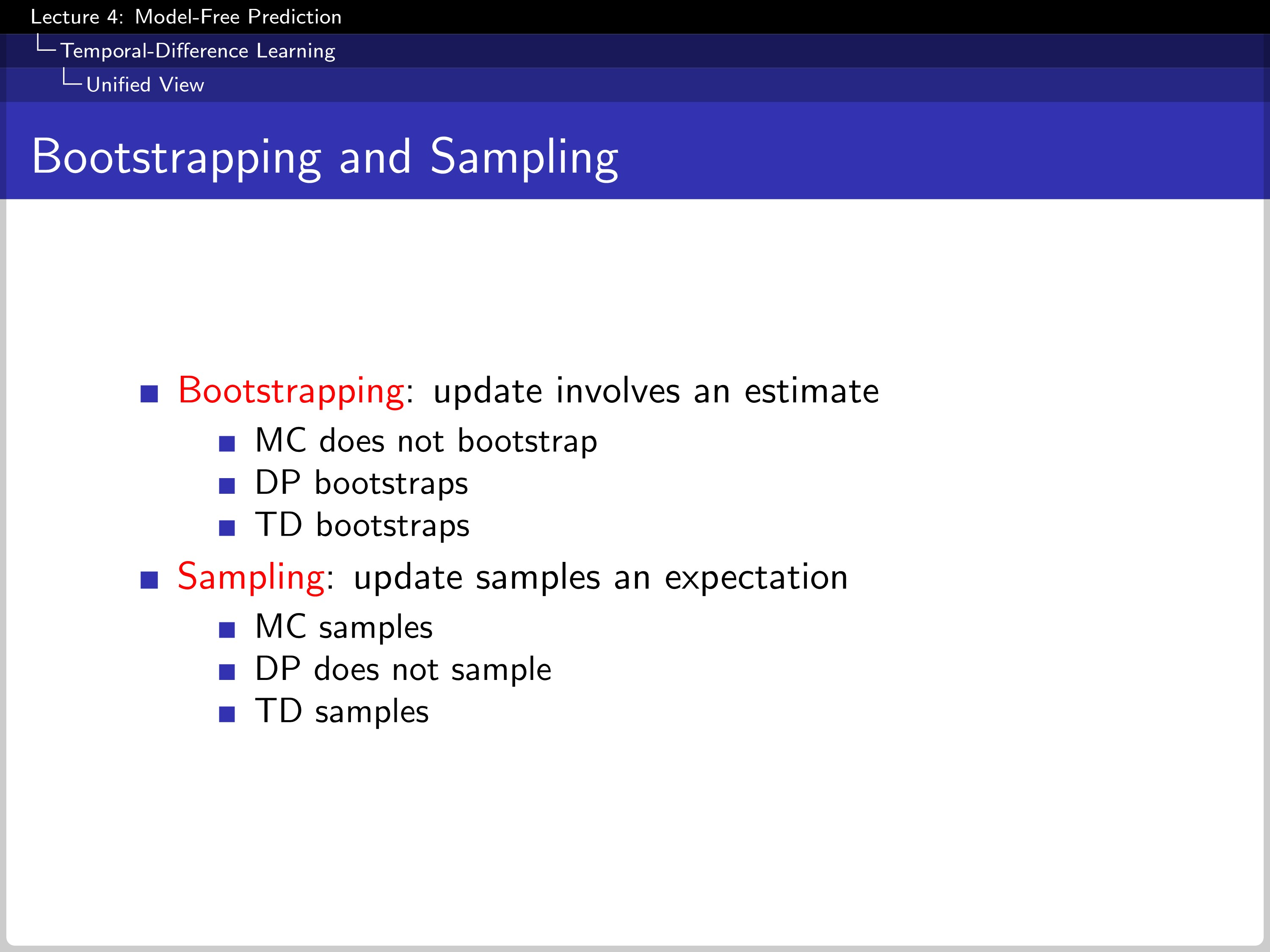
Bootstrap contains estimates in an update process. In this point of view, MC does not bootstrap, but DP and TD do bootstraps. This can be rewritten as a bootstrap check shallower range than MC. In sampling, MC and TD do samples. But DP does not because it knows the whole transition data of MDP.
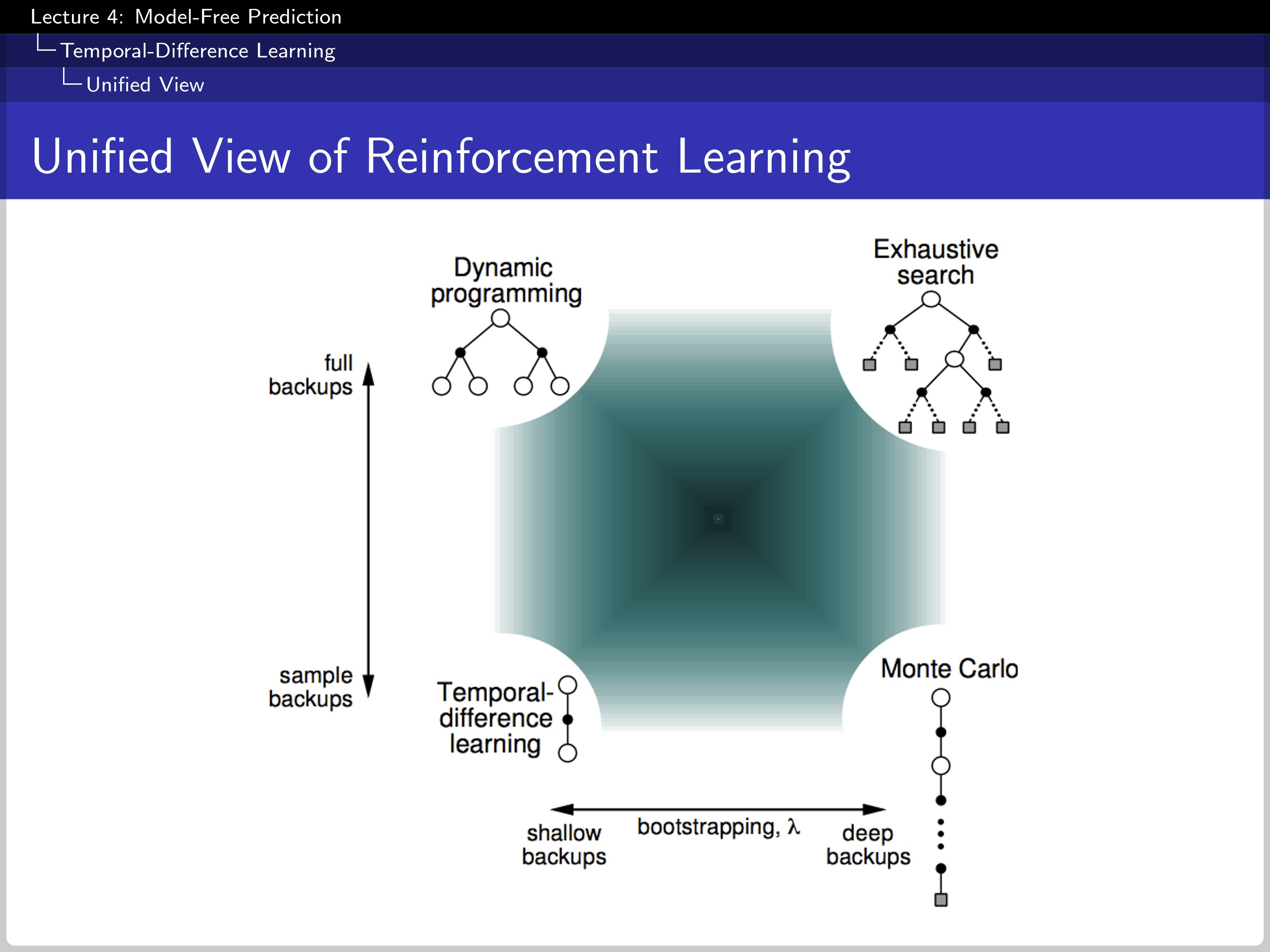
It shows the overall position of each algorithm; Y-axis shows if the algorithm use sampling and X-axis show if the algorithm use bootstrapping.
n-step TD
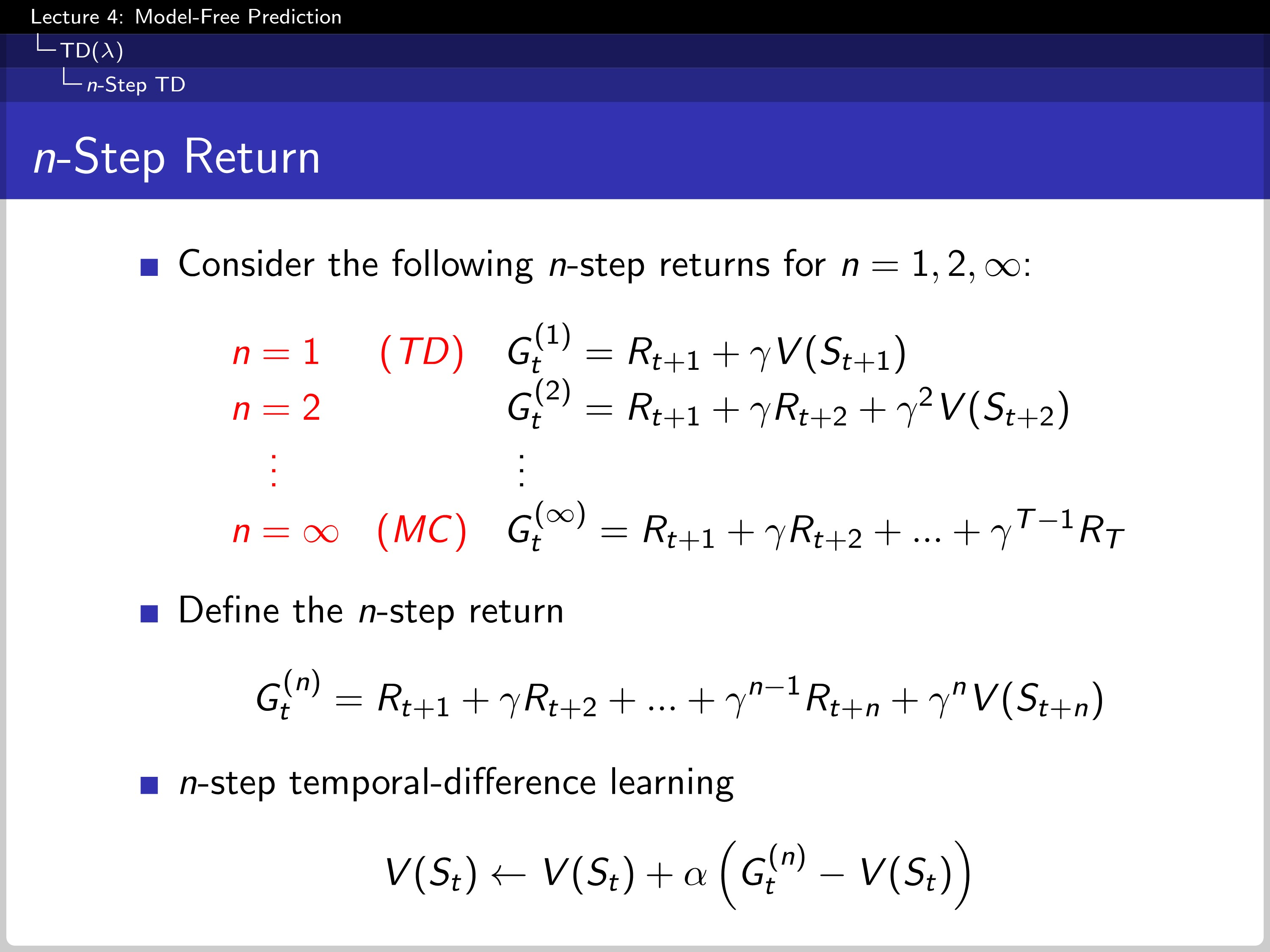
TD algorithm can be modified by using n-step TD. For example, maximum n means it uses MC. with n as a value of 1; the TD becomes a 1-step TD, which is TD(0).
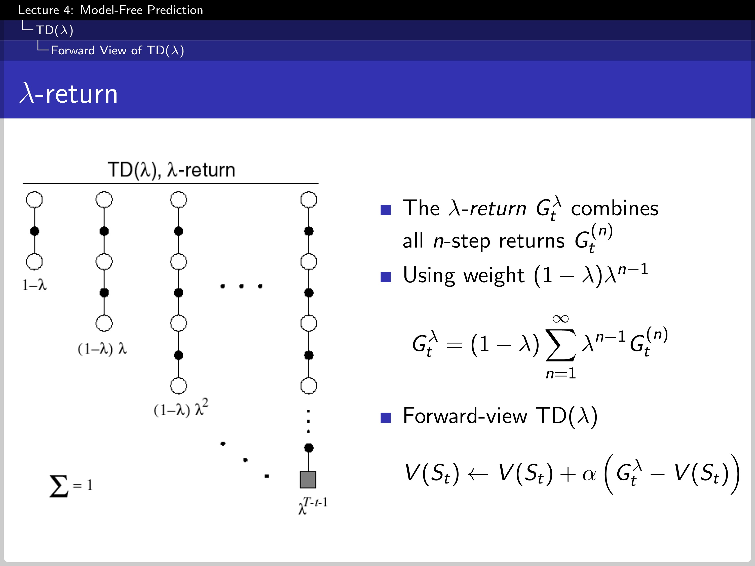
We average the return by multiplying $\lambda$ at G, a geometric mean of $G_{t}$. Using forward-view TD($\lambda$) and $G_{t}^{\lambda}$. This formulation has an advantage in calculation complexity, which has the same complexity as TD(0), but has a drawback in it needs a full memory of future returns. It also requires ending the whole episode.
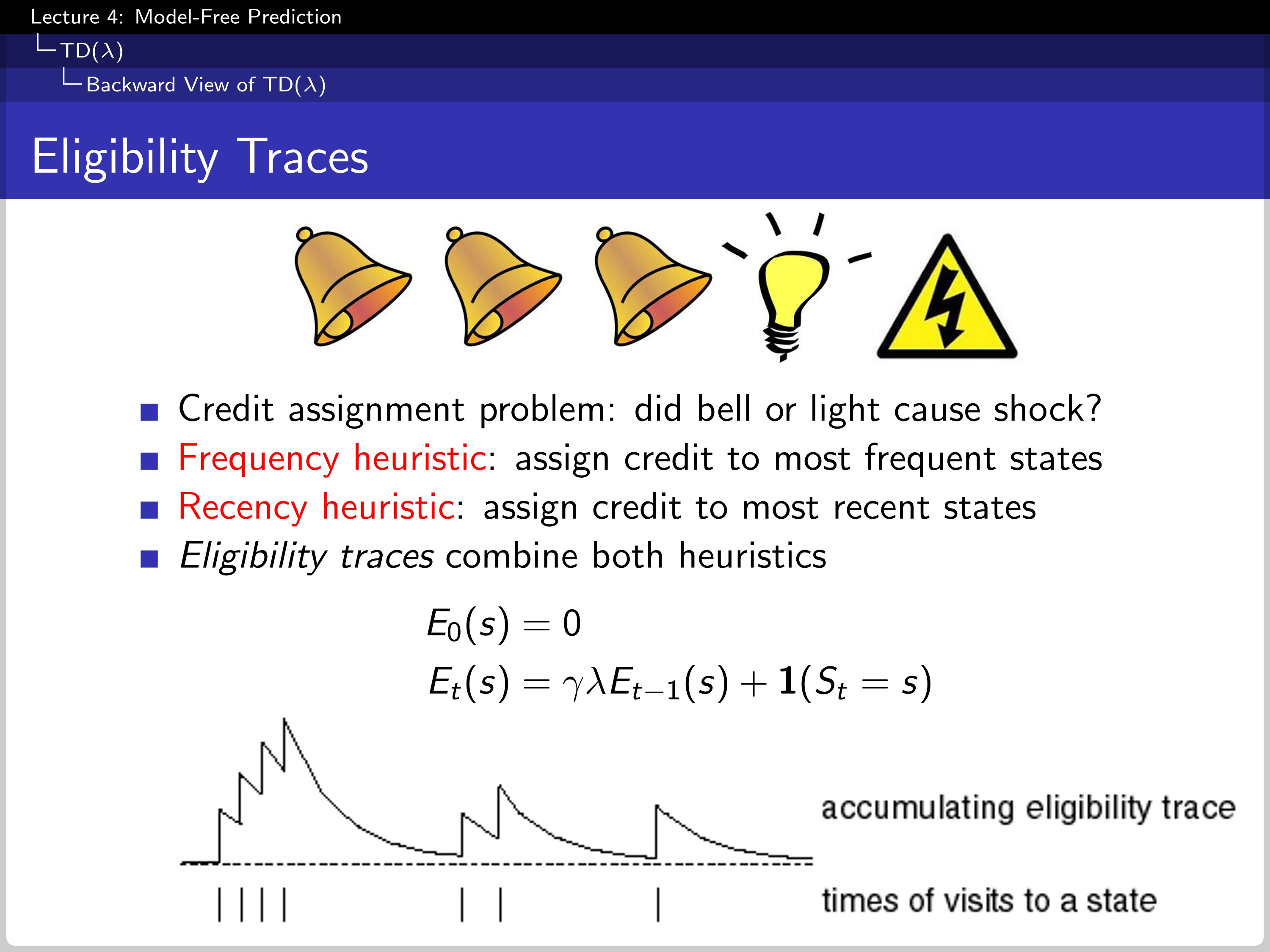
To handle this drawback, we use the eligibility traces. The eligibility decreases geometrically because the $\gamma$ is multiplied at each time step and added by one if the agents visits the state.
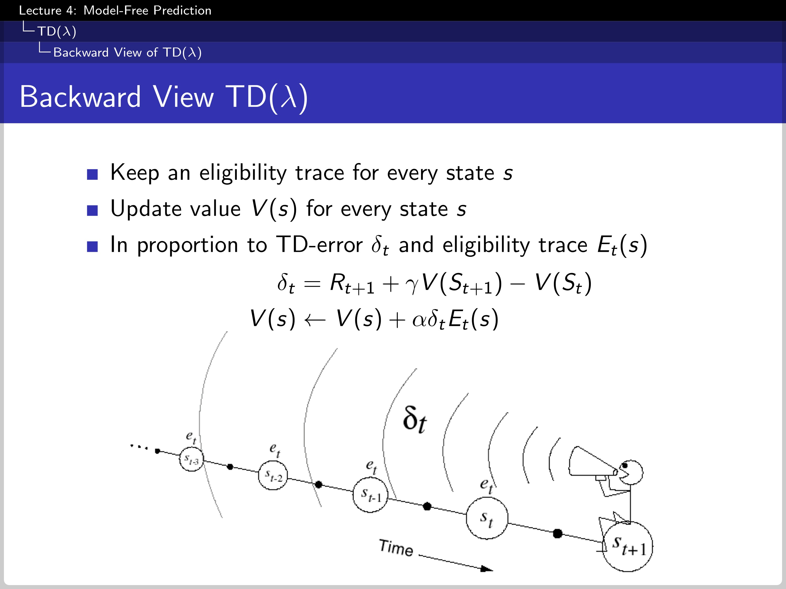
Using the eligibility trace, we can change forward view TD($\lambda$) to backward view TD($\lambda$).
The Relationship Between Forward and Backward TD
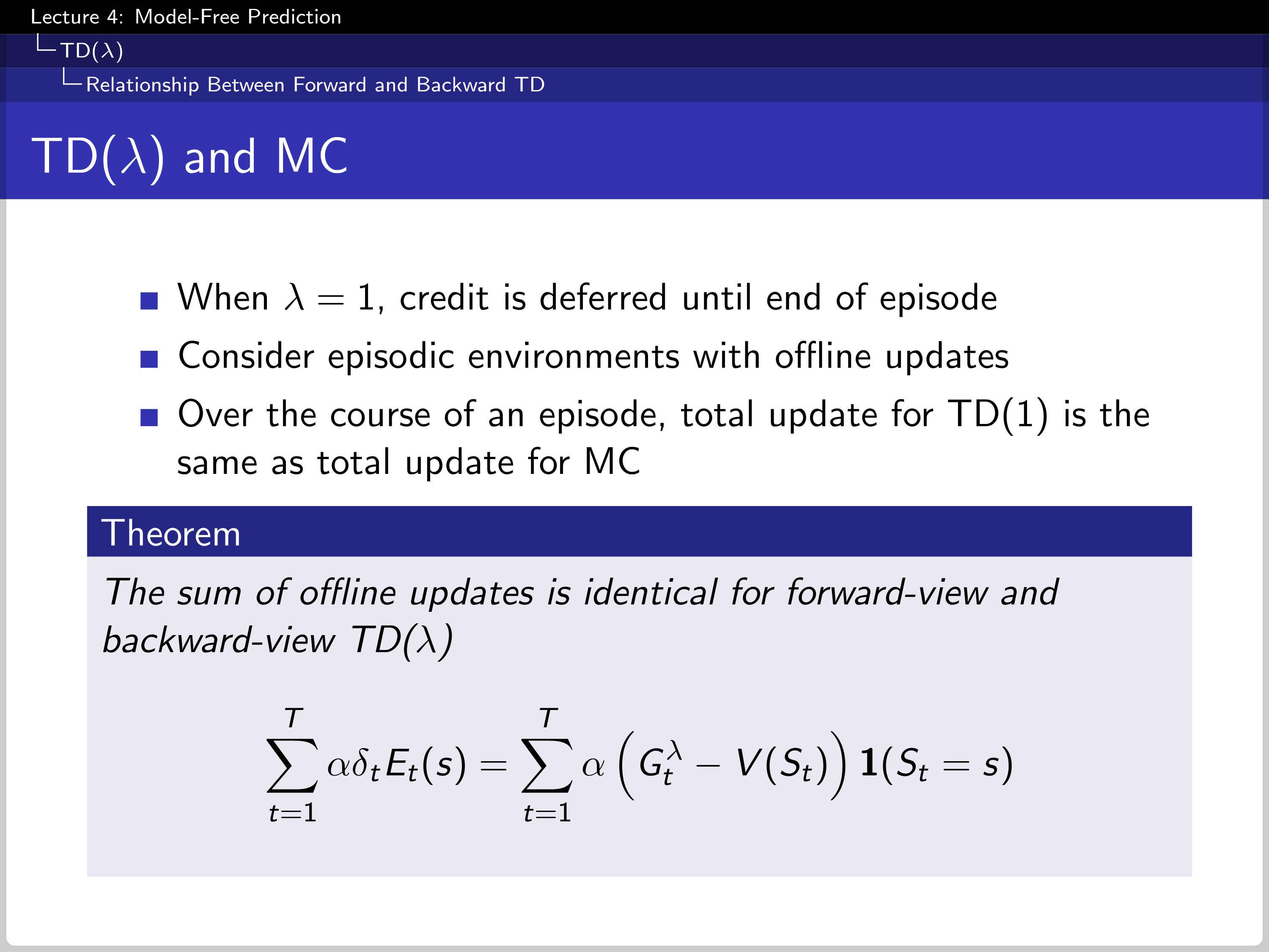
The theorem shows the sum of the offline updates is identical for forward-view and backward-view TD($\lambda$).
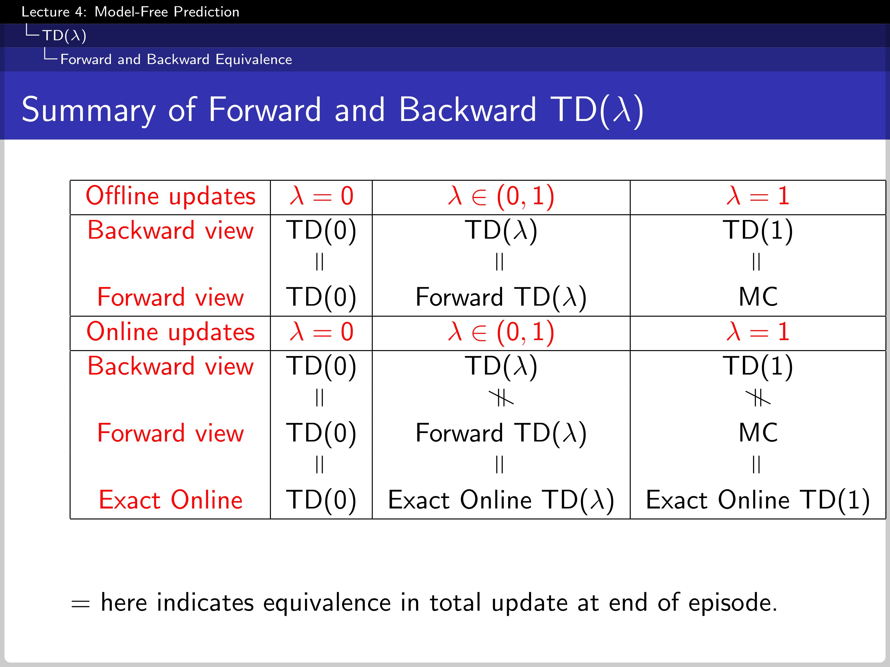
The chart summarizes the result.


